As previous articles have discussed, investors and analysts often use historical and projected dividend payments to estimate the intrinsic value of a stock. While simpler models, like the Gordon Growth Model and the two-stage dividend discount model, offer ease of calculation and interpretation, they rely on broad assumptions about dividend performance – namely, that dividends will grow at a constant rate. While the two-stage model does account for a shift in dividend growth, this change is assumed to occur instantaneously at the end of a period of aggressive but stable dividend growth.
In reality, most companies either reduce or increase dividends over time rather than dramatically shifting gears from high yields to stable growth. The H model was developed to estimate the value of a firm whose dividend growth rate is predicted to change, but not all at once.
What Is the H-Model?
The H-Model dividend discount formula is like the two-stage model in that it calculates the present value of dividends in two key phases. However, whereas the two-stage model assumes dividends will grow at one rate and then suddenly drop to a lower rate for the foreseeable future, the H-Model accounts for the gradual change in dividend rates over time.
In the first phase of the H-Model calculation, dividends are assumed to increase or decrease in regular increments each year. For example, a company’s dividend growth rate may decline by 2% each year for three years to transition from 15% to 9%. The rate of change remains consistent but the growth rate itself gradually decreases.
The second stage of the H-Model is identical to that of the two-stage model or the Gordon Growth Model. During the first phase, the growth rate slowly changes until it stabilizes at the growth rate that will be maintained over the life of the company. In the example above, the fourth year would see dividend growth reduced to 7%, where it would stabilize. The Gordon Growth Model formula can be used to calculate the present value of all future dividends based on this stable 7% increase per year.
Discount Models and the Time Value of Money
Like the two-stage, three-stage, and Gordon Growth models, the H-Model is a valuation formula that discounts future cash flows using an expected rate of return to account for the time value of money. A dollar earned a year from now is worth less than a dollar earned today because funds you have today can be invested to generate interest over the coming year, while money you have to wait for cannot. The time value of money, therefore, means that each subsequent dividend dollar is worth less today than the one before it because you have to wait longer to receive it.
Because dividend discount models are predictive by nature, they use the required rate of return or cost of equity to discount future dividend payments and render the present value of a stock after accounting for the time value of money.
The H Dividend Discount Model Formula
As a dividend discount valuation formula becomes more precise, it also becomes more complex. However, the basic components of this formula remain simple to understand and easy to assemble. All that is needed are the initial growth rate, the final rate at which dividend growth will stabilize after transitioning from the current rate, the period over which the rate will change, the expected rate of return, and the amount of the dividend payment to be paid one year from today.

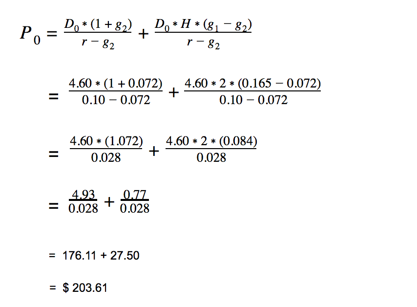
In this formula, D0 is the current year’s dividend payment, g1 and g2 are the initial and terminal growth rates, respectively, r is the expected rate of return and H is equal to half of the anticipated transition period.
Example
Lockheed Martin (LM ) the aerospace and defense conglomerate, has a stellar dividend history, with steadily increasing quarterly payments since 1995. In recent years, however, the rate of dividend growth has declined from a solid 15.6% in 2014 to 10% in 2016. Of course, the 2016 fiscal year has just begun as of this writing, but the total dividend can be extrapolated from the first quarter dividend of $1.65 per share and the company’s history of consistent quarterly payments.
Based on this steady rate of decline, it can be assumed that dividend growth will again decrease by 2.8% in 2017 and then stabilize at a healthy 7.2% thereafter. This example will use LMT’s actual dividend performance for 2013 through 2016, along with a projected decline and stabilization in 2017, to produce a value estimate for the stock in 2013 using the H model dividend discount calculation. For the purposes of this example, a 10% expected rate of return is used. The number of years over which the growth rate will transition is four, so H = 2.
By plugging the above information into the H-Model equation, you can easily calculate the value estimate using the 2013 dividend payment of $4.60.

With the proper information, this equation is relatively straightforward. However, a clear understanding of what these numbers mean is key to harnessing the power of these predictive models and to properly interpreting the results. To this end, let’s break down this calculation into its component parts.
In the first phase of dividend growth, the growth rate declines by 2.8% each year for four years, beginning with the 2013 dividend payment of $4.60. The first step, therefore, is to determine the value of these ‘projected’ dividends for the 2014 through 2017 fiscal years.
- D2014 = $4.60 * 1.156 = $5.32
- D2015 = $5.32 * 1.128 = $6.00
- D2016 = $6.00 * 1.100 = $6.60
- D2017 = $6.60 * 1.072 = $7.08
Next, use the stable rate of growth from 2017 onward to determine the total value of all future dividends using the Gordon Growth Model formula.
- VDFuture = D2017 / (R – G2)
- VDFuture = $7.08 / (0.10 – 0.072)
- VDFuture= $7.08 / 0.028
- VDFuture = $252.86
Now, calculate the present value of all future dividends by applying the discount rate.
- PVD2014 = $5.32 / (1 + 0.10)1 = $4.84
- PVD2015 = $6.00 / (1 + 0.10)2 = $4.96
- PVD2016 = $6.60 / (1 + 0.10)3 = $4.96
- PVDFuture = $252.86 / (1 + 0.10)3 = $189.98
Finally, sum the present values of all future dividends to render the intrinsic value of LMT’s stock in 2013.
- Stock Value = $4.84 + $4.96 + $4.96 + $189.98 = $204.74
A small difference between calculations is to be expected due to the rounding error inherent in hand calculations. Whenever possible, using an online calculator or spreadsheet formula will yield more exact results.
Interpretation
The actual value of Lockheed Martin’s stock as of October 2, 2015, is $206.61 – almost exactly the value this model predicts. In fact, the stock’s price has been rising steadily for the past several years, indicating that investors feel the company will remain profitable for years to come.
However, this model was meant as a predictive calculation to determine whether or not LMT would have been a good investment back in 2013 based on dividend projections. In 2013, the stock’s price increased from $93 to $148 per share, meaning it would have been substantially undervalued based on this model. Though there would be no way to know for sure if the prediction was correct, an investor that bought shares of LMT based on these calculations would certainly be a happy camper today.
Since this example used LMT’s actual dividend data, it can be inferred that investors and analysts alike are interpreting the recent dividend changes in the same way. Especially given the stock’s track record for consistent capital gains, the current price is right on target – if slightly generous – if its valuation is based on the assumption that dividend growth will continue to decline for another year, before stabilizing around 7%. Only time will tell what the actual dividend performance will be, but this example perfectly illustrates the predictive power of dividend discount modeling.
Check out the Dividend Discount Model, the Two-Stage Dividend Model and the Three-Stage Dividend Model.
Image courtesy of Matt Banks at FreeDigitalPhotos.net


